McCal: Matrix Calculation

McCal Matrix Calculation

In this document, we explain how to conduct matrix calculation in McCal. McCal has a powerful set of operators and functions to handle matrix calculation.

McCal Version 4.3 now supports MATLAB (registered trade mark of MathWorks)-like operators.

There are two ways to define a matrix in McCal. The first method is to use the box brackets and Dim (dimension) statement. The other is ArrayViewer, in which users can define matrix data interactively. We describe the box bracket method in this chapter.

A matrix can be defined by listing the values for its elements using commas and a pair of box brackets. Please use nested brackets to indicate the rows of the matrix.

a = [1,2,3,4]
▶︎ array[4]
Print a
▽1  ▽2  ▽3  ▽4

a = [[2,3],[1, -1+2i]] 
▶︎ array[2][2]
Print a
▽2　▽3
▽1　▽-1+2i

Print a+a
▽4　▽6
▽2　▽-2+4i
▶︎ array[2][2]

In the present implementation of McCal, the expression must be in one line. Line breaks are not allowed in the box bracket statement.

Dim statement declares the sizes of the matrices.

Dim a[3][3] = [[2,3],[1,-1]] 
Print a
▽2  ▽3  ▽0
▽1  ▽-1 ▽0
▽0  ▽0  ▽0
▶︎ array[3][3]

McCal now supports the colon operator, with which a 'start', 'incremental' (optional), and 'end' values are indicated. The incremental value is assumed to be '1' (one), if it is omitted. The colon operator is also expained later.

c = 1:5
Print c
▽1  ▽2  ▽3  ▽4  ▽5
▶︎ array[1][5]

c = 1:0.1:1.4
Print c
▽1  ▽1.10  ▽1.20  ▽1.30  ▽1.40
▶︎ array[1][5]

Plese not that, in the above example, the size of the returned array is '1 x N'. In other words, it's a 2D array with only one row. Please use the transposition operator (', dash) to convert it to vector (1D matrix), if you want.

Print c'
▽1  ▽1.10  ▽1.20  ▽1.30  ▽1.40
▶︎ array[5]

Box brackets notation can be used as a matrix in an expression. In other words, it can be an operand of an operator, or passed to a function.

Print [[2,0],[0, 2]] * [[#cos(30), -#sin(30)],[#sin(30),#cos(30)]] 
▽1.7321  ▽1.0000
▽1.0000  ▽1.7321
▶︎ array[2][2]

Using ArrayViewer, users can define the values of the elements of a matrix. First, please declare a matrix (its size can be changed in ArrayViewer):

Dim @soccer[5][5]

Pressing the ViewerIcon button in the Android ActionBar activate the McCal Viewer. Then select 'soccer' under "Variable" tab. ArrayViewer starts up.

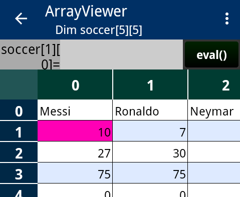
Double-tap on the cell you like to change, and the cell is activated (the backgraound color is changed to red). Enter an expression , and then press eval() button. The evaluated value will be entered in the cell.

Please see ArrayViewer Help for more information.

Array index is used for accessing the matrix element of your interest. Box brackets are used as follows. Please note that both 'c[1,2]' and 'c[1][2]' are allowed.

Print c
▽1.7321  ▽1.0000
▽2i  ▽1.4142
▶︎ array[2][2]

c[0][0]
▶︎ 1.7321

c[1,0]
▶︎ 2i

As described before, box brackets are also used for defining a matrix. McCal assumes that the box brackets just after a variable name are for array indexing. In other words, to get a specific element of a matrix by indexing, first ubstitue an appropriate vaiable with the matrix data.

Since version 4.3, the colon operator can be used for obtaining a specific region of a matrix. The colon operator is explained in McCal Help document. In the following example, we use an array, c.

Print c
▽1.7321  ▽1.0000  ▽0.0000 
▽1.0000  ▽0.5000  ▽i
▽-12345  ▽0.0000  ▽1.0000 
▶︎ array[2][2]

Print c[1:2][1:2]
▽0.5000  ▽i
▽0.0000  ▽1.0000 
▶︎ array[2][2]

c[:,0]
▽1.7321  ▽1.0000  ▽-12345
▶︎ array[3]

Following examples are for addtion/sustraction, multiplication of matrix.

Dim a = [[2,3],[1,-1]] 
Print a+a
▽4  ▽6
▽2  ▽-2

Print a=a*a
▽7  ▽3
▽1  ▽4

Dim b=[1,0]
Print ab
▽7  ▽1

The two matices must be the same size in addition and substraction. In the case of matrix multiplication, the number of the row elements of the first matrix must be the same to that of the vertical elements of the second. 1D arrays (vectors) are treated as a matrix with only one column; in the above case, 'b' is assumed as a 2x1 matrix.

Element-by-element operations

McCal now supports some element-by-element operators, such as multiplication and division. The dot character for these two-character operators can be entered using the floating point button ( . ) in the number pad of McCal.

Dim a=[[2,3],[1,-1]], b=[[2,1],[3,i]]
Print a
▽7  ▽3
▽1  ▽4
Print b
▽2  ▽1
▽3  ▽0+i

Print a.*b
▽14  ▽3
▽3   ▽0+4i

Here is a list of the McCal operators for Matrix calculation.

Operator	Name	Description
A/B	Right division	Same as multiplication of the inverse of B from right. B must be a square, regular matrix.
A\B	Left division	When A*x=B, x=A\B. Same as multiplication of the inverse of A from the left.
A./B	Right array division	Each element of A is divided by the corresponding element of B. A and B must be the same size, or either one is a scaler.
A.\B	Left array division	Each element of B is divided by the corresponding element of A. A and B must be the same size, or either one is a scaler.
A'	Conjugate transposition	Returns the complex conjutate of the transpose of A.
A.'	Array transposition	Returns the transpose of A.
A.^B	Array power	Returns the matrix in which each element is A[i,j]^B[i,j]. A and B must be the same size, or either one is scaler.
A.*B	Array multiplication	Each element of A is multiplied by each element of B. A and B must be the same size, or either one is scaler.

(Mx) button brings up a short cut to some of these operators.

When A is a square matrix, power oerator (^, x^y ) calculates the power of the matrix. The second operand (index) must be integer larger or equal to -1.

Dim b=[[2,1],[3,i]]
b^(3)
▽20+3i　▽6+2i
▽18+6i　▽6+5i
▶︎ array[2][2]

When the index is 0 (zero), power operator returns the identity matrix of the same size. This is the simplest way to obtain the identity matrix in McCal.

Dim b=[[2,1],[3,i]]
I = b^(0)
Print I
▽1　▽0
▽0　▽1
▶︎ array[2][2]

When the index is -1, the power operator returns the inverse of A.

>Dim b=[[2,1],[3,i]]
Print b^(-1)
▽0.1538-0.2308i　▽0.2308+0.1538i
▽0.6923+0.4615i　▽-0.4615-0.3077i
▶︎ array[2][2]

Let's test it.

>Dim b=[[2,1],[3,i]]
Print b*b^(-1)
▽1.0000　▽0
▽0　▽1.0000-0i
▶︎ array[2][2]

Sometimes the result contains rounding error (approximatel < 1×10^-13)

It is easy to solve simultaneous equations with McCal, even if its coefficients contain complex numbers.

Example

x＋２y＋３z＝１４
２x−y＋２z＝６
３x−２yーz＝−４

These equations can be expressed as follows using matrices.

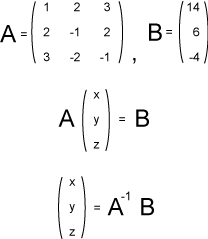
Therefore, let's define the matrices:

A = [[1,2,3],[2,-1,2],[3,-2,-1]]
B = [14,6,-4]

We use the left-division operator, here.（x = A^-1B = A\B).

Print A\B
▽1.0000　▽2.0000 ▽3.0000
▶︎ array[3]

The answers are 1, 2, 3, respectively, although McCal uses floating point numbers.

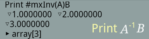
It7s possible to obtain the inverse of matrix A using power operator.

Print A^(-1)*B
▽1.0000　▽2.0000 ▽3.0000
▶︎ array[3]

The following example uses the inverse function.

This chpter is about the eignvectors and eigenvalues function, #mxEig(A). The argument for this function must be a square matrix of which elements are real numbers.

This function calculates and returns eigenvectors and eigenvalues in two matrices. Some matrix has complex eigenvalues. McCal can handle complex eigenvalues and eigenvectors.

What is eigenvector?

Av = λv ……… (1)

An eigenvector (v in above equation) of a sqaure matirx (A, above) is a vector that does not change its direction under the associated linear transformation of A. Here, the scaler value λ is called eigenvalue of vector v. In some cases, λ can be a complex number.

Calculation of Eigenvectors and eigenvalues is often required in some fields of engineering and science.

#mxEig(A) returns two matrices. Please use box brackets to capture these matrices.

  [V,D] = #mxEig(A)

Example 1:

 Print A
   ▽ 1  ▽ 2  ▽ 3
   ▽ 2  ▽ 3  ▽ 1
   ▽ 3  ▽ 1  ▽ 2

 [V,D] = #mxEig(A)
 Print V
   ▽ 0.5774  ▽ 0.7317 +0.3624i ▽ 0.36237 -0.73168i
   ▽ 0.5774  ▽ -0.6797 +0.4525i ▽ -0.6797 -0.4525i
   ▽ 0.5774  ▽ -5.2021E-2 -0.8148i ▽ -5.2021E-2 +0.8148i

 Print D
   ▽ 6.00000 ▽ 0  ▽ 0
   ▽ 0 ▽ -1.5000 -0.8660i  ▽ 0
   ▽ 0 ▽ 0  ▽ -1.5000 +0.8660i

Eigenvalues are listed in the diagonal elements in the matrix for eigenvalues (D). Eigenvectors are stored in the vertical columns of the matrix (V).

Let's test the first eigenvector, [0.5774, 0.5774, 0.5774]. We use the colon operator to get the first colomn of matrix V.

Print A*V[:,0] - D[0,0]*V[:,0]
▽0  ▽0  ▽0

From eq. 1, V and D should have the following relation.

AV = VD ……… (2)

If V is a regular, (in this case, yes)

V^-1AV = D ……… (3)

Let's test eq. 3

 Print V^(-1)*A*V
   ▽ 6.00000 ▽ 0  ▽ 0
   ▽ 0 ▽ -1.5000 -0.8660i  ▽ 0
   ▽ 0 ▽ 0  ▽ -1.5000 +0.8660i

For more information about eigenvectors and eigenvalues, please see Wiki page (external link).

While every effort is made to ensure the correct operation and accuracy, MilimaCode cannot be held responsible for any errors resulting from its use.

McCal Matrix Calculation

1.　Introduction

2.1　Defining a matrix

2.2　ArrayViewer

2.1　Getting an element

2.2　Getting elements: colon operator

3 Matrix calculation

3.1 Matrix operators

3.2 Power of Matrix.

3.3　Simultaneous Equations

3.4 Eigenvectors and Eigenvalues

4 Disclaimer

McCal Matrix Calculation

1. Introduction

2.1 Defining a matrix

2.2 ArrayViewer

2.1 Getting an element

2.2 Getting elements: colon operator

3 Matrix calculation

3.1 Matrix operators

3.2 Power of Matrix.

3.3 Simultaneous Equations

3.4 Eigenvectors and Eigenvalues

4 Disclaimer

1.　Introduction

2.1　Defining a matrix

2.2　ArrayViewer

2.1　Getting an element

2.2　Getting elements: colon operator

3.3　Simultaneous Equations