Polynomial functions and Equation solver
In this document, we explain how to calculate polynomials and to solve polynomial equations.
What is Polynomial?
Polynomial is an expression consisting of the addition, subtraction, multiplication of coefficients and non-negative exponents of variables. For example, the following expression is a 4-order polynomial of variable 'x'. Here, a4 ~ a0 are the coefficients of the polynomial.
a4x4 + a3x3 + a2x2 + a1x + a0
McCal has a rich set of functions for handling polynomials, such as multiplication, devision, and equation solver.
How is Polynomial treated in McCal?
In McCal, 1-dimensional arrays (vectors) of coefficents are used to represent polynomials of single variable, ordered by descending power. In the above case, polynomial functions of McCal take [a4, a3, a2, a1, a0] as the polynomial argument.
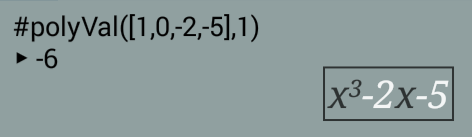
For example, [1,0,-2,-5] is utilized to represent the following polynomial p(x).
p(x) = x3 - 2x - 5
In the screen-shot below, the coefficient array is passed to a McCal function called #polyVal(), to calculate the value of polynomial at x=1. The result is p(1)= -6.
The names of the McCal functions for handling polynomials start with "#poly". The documents of these functions are organized in the "Polynomial" under "System Function" of FunctionViewer.
Natural Display
In the example of the previous chapter, the polynomial is in "Natural-Display" at the lower-right corner of the screen shot. It is placed in a black box.
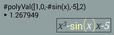
McCal uses 'x' for the variable of the polynomial in 'Natural-Display'. Please note that McCal uses black color for 'x', in order to show it's different from McCal memory, 'x', as shown in the following screen-shot.
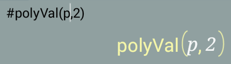
In the above cases, the cofficient arrays were provided with box brackets, "[, ]". When a variable is used for the cofficient data, McCal uses 'Natural-Display' similar to other system functions. In the example below, 'p' hold the coefficients data.
Solving equations
McCal has a special function, #polySolv(), for solving polynomical equations. It takes a single argument for the coefficient array of the polynomial equation, and returns the roots of the equation in the vector format. We explain #polySolv() using examples.
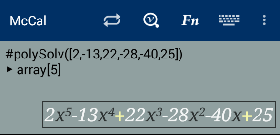
Example 1
2x5 -13x4 + 22x3 = 28x2 + 40x - 25
First, move all elements to the left side of equation, so that the equation is something like f(x) = 0.
2x5 -13x4 + 22x3 - 28x2 - 40x + 25 = 0
Next, just pass the corresponding coefficient array to #polySolv(). It returns the roots in an array.
#polySolv([2, -13, 22, -28, -40, 25])
  ▶︎ array[5]
Just Press button to view the content of the array, -1, 0.5, 1-2I, 1+2i, and 5.
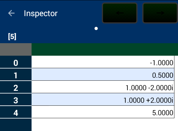
Or use the 'Print' command instead, as shown below.
 Print #polySolv([2, -13, 22, -28, -40, 25])
▽-1.000 ▽0.500 ▽1.000 -2.000i ▽1.000 +2.000i ▽5.000
  ▶︎ array[5]
Testing the roots
Let's test the roots obtained in the previous chapter.
p = [2, -13, 22, -28, -40, 25]
First, save the coefficients in an array 'p' for later-reuse. Next, save the roots in a variable, 'a'.
 a = #polySolv(p)
  ▶︎ array[5]
 Print a
 ▽-1.000 ▽0.500 ▽1.000 -2.000i ▽1.000 +2.000i ▽5.000
We calculate the value of polynomial, p(x), for each root using #polyVal() . When the second argument of #polyVal() is an array (xi,j), it just returns the array of which element is the value of polynomial, p(xi,j).
 Print #polyVal(p, a)
 ▽ 0 ▽0 ▽0 +0i ▽0 ▽ -9.202E-13
 ▶︎ array[5]
As shown above, each element is almost zero, although it contains rounding errors between 10-12 ~ 10-14.
Testing the roots, #2
In the example in the previous chapter, the returned array seems to include -1, 1/2, and 5. Let's divide the original polynomical with (x+1)(2x-1)(x-5). The remainder of the division should be zero, if -1, 1/2, and 5 are the roots of the polynomial equation.
 Print #polyDiv(p, #polyMul([1,1],[2,-1],[1,-5]))
 ▽1  ▽-2  ▽5

 ▽0
 ▶︎ array[3], 0
#polyDiv() returns the quotient and remainder. As shown above, the remainder is zero. Thus,
2x5-13x4+22x3-28x2-40x+25 = (x+1)(2x-1)(x-5)(x2-2x+5)
List of McCal functions for handling polynomials
The names of the system functions start with "#poly." The documents are organized under FunctionViewer→"System Function"→"Polynomial". Here is a summary of some functions.
Polynomial value #polyVal(p,x): Returns the value of p(x). When the second argument is an array (xi,j), this function returns the array of which element is p((xi).
Addition, subtraction, multiplication, division #polyAdd(a, b), #polySub(a, b), #polyMul(a, b), #polyDiv(a, b).
Solving the given polynomial equation: #polySolv(p).
Derived function: #polyDer(p).